
As of Monday, December 21, 2026, DDx will adjust scoring for all rubric-based cases on a go-forward basis. Cases completed on or after December 21st use the adjusted score, and cases completed before that date keep their original score.
If you want every score in your gradebook on one scale, you can convert scores yourself in Excel or Google Sheets. This article covers two options:
Option A: Convert past scores (completed before December 21st) to the adjusted model.
Option B: Convert new scores (completed on or after December 21st) back to the previous model.
Before you start
You'll need instructor or admin access to the DDx Performance page and a spreadsheet program such as Microsoft Excel or Google Sheets.
Export your scores
These steps are the same for both options.
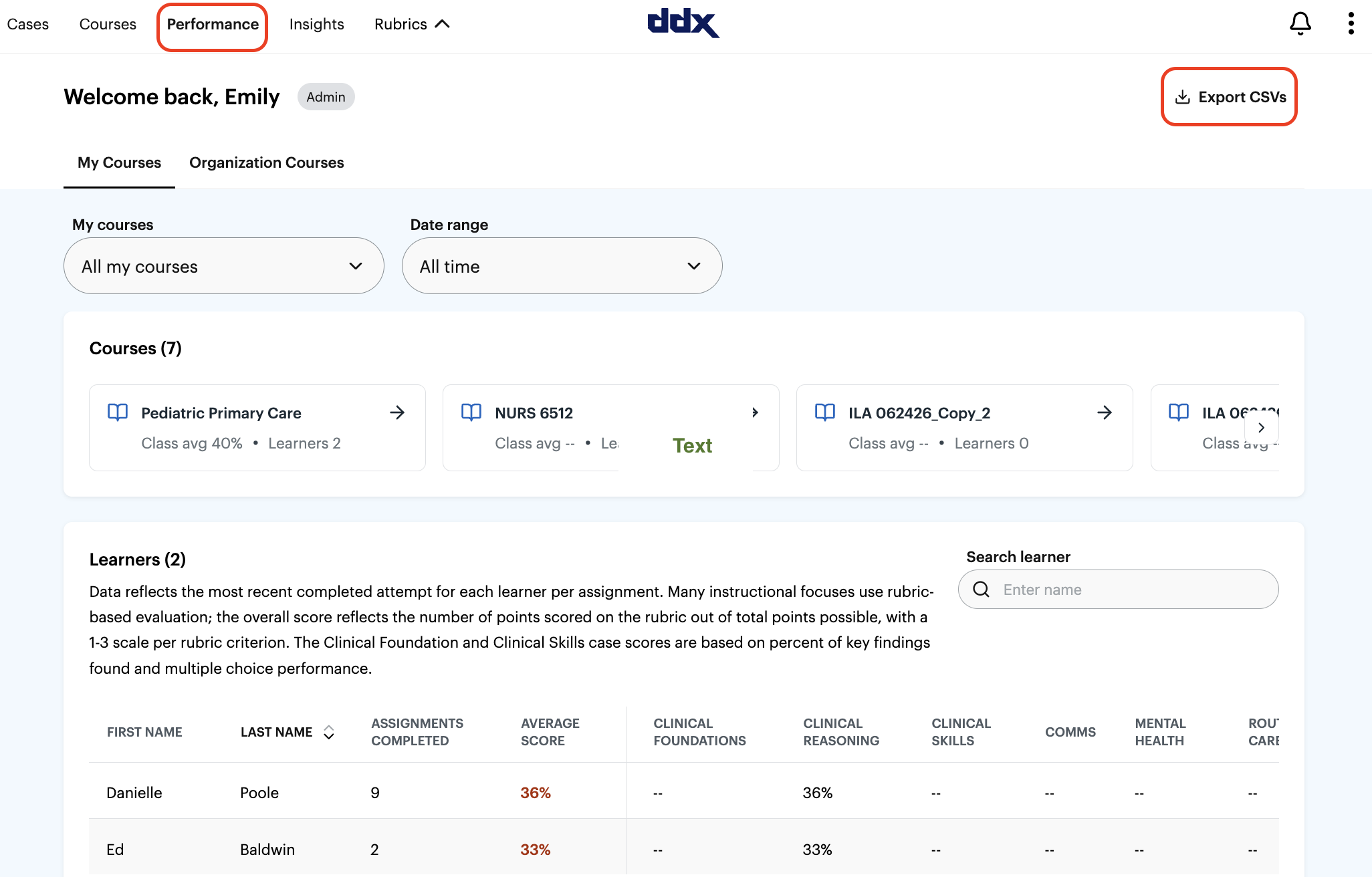
In DDx, select Performance in the top navigation.
Use the My courses and Date range filters to select the course and time period you want to convert.
Select Export CSVs in the top right corner of the page.
Open the file named ddx-assignment-performance in Excel or Google Sheets. Every DDx assignment performance export uses the same column layout, so the formulas below work in any file you download. These are the three columns you'll use:
Column | Header | What it contains |
|---|---|---|
F | Rubric Type | The rubric used for the case, or "No rubric" |
G | Case Score | The learner's score as a whole number (for example, 33 means 33%) |
O | Completed At | The date and time the learner completed the case, in UTC |

Option A: Convert past scores to the adjusted model
Use this option if you want scores from before [launch date] to match the adjusted scores DDx reports today.
Turn on filters for the header row (in Excel, Data > Filter; in Google Sheets, Data > Create a filter).
Filter column F (Rubric Type) to hide rows marked No rubric. Keep every other rubric type selected.
Filter column O (Completed At) to show only cases completed before December 21. 2026.
In the first empty column to the right of your data, type the header Adjusted Score in row 1.
In row 2 of that column, enter or copy/paste this formula:
=ROUND(40+0.6*G2,0)
Copy the formula down to the last row of filtered data.
For example, a past score of 33 converts to 60, a score of 67 converts to 80, and a score of 83 converts to 90.
Option B: Convert new scores to the previous model
Use this option if your course is already graded on the previous scale and you want to keep it that way through the end of the term.
Turn on filters for the header row (in Excel, Data > Filter; in Google Sheets, Data > Create a filter).
Filter column F (Rubric Type) to hide rows marked No rubric. Keep every other rubric type selected.
Filter column O (Completed At) to show only cases completed on or after December 21, 2026.
In the first empty column to the right of your data, type the header Previous Model Score in row 1.
In row 2 of that column, enter or copy/paste this formula:
=ROUND((G2-40)/0.6,0)
Copy the formula down to the last row of filtered data.
For example, an adjusted score of 60 converts to 33, a score of 80 converts to 67, and a score of 90 converts to 83.
Tip
Save as a spreadsheet file. CSV files don't keep formulas. Before closing, save your work as an Excel workbook (.xlsx) or keep it in Google Sheets.
Need help?
If you'd like help converting scores or deciding which option fits your course, email institutionalsupport@sketchy.com. Our team can walk through the steps with you or help plan your transition to the adjusted score.